

What is Semantic Search?
How Machines Started Understanding Meaning

🧭 Part 7 of RAG & Search course
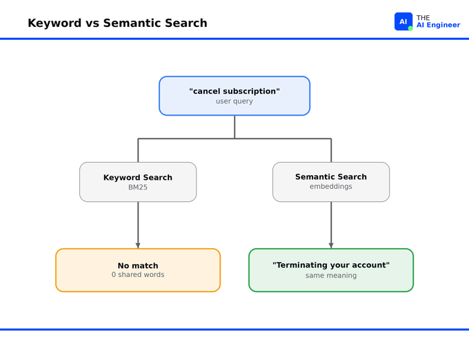
A customer types “cancel subscription” into your help search. Your top-ranked article is titled “Terminating your account,” updated three days ago by your billing team. The search returns nothing. The customer files a ticket. Your support team has logged those tickets as “search bugs” for six months. They are not bugs. Keyword search is matching the literal tokens you typed, which is all keyword search ever does.
TL;DR
Semantic search retrieves by meaning. Your query becomes a vector, your documents become vectors, and the system returns whichever document vectors sit closest to the query. The match works even when zero words overlap between query and document.
Hybrid search beats pure semantic. Every serious 2026 search system runs semantic alongside BM25, fuses the rankings with Reciprocal Rank Fusion, and reranks the top 100 results with a cross-encoder.
The hard decisions are model choice, chunking, and cost. The wrong embedding model costs 10 to 30 points of retrieval accuracy on specialized verticals. The wrong chunking strategy caps retrieval quality no matter how good the model is. And every query now costs an embedding call plus a vector search plus a rerank, paid in latency and dollars.
Reranking with a cross-encoder is the next quality jump after hybrid. A bi-encoder retrieves the top 100 in ~5ms, a cross-encoder rescores them in ~50ms. Cohere Rerank, BGE Reranker, and ColBERTv2 are the production defaults.
First, Keyword Search, and Why It Falls Short
The simplest mental model is a library card catalog. You walk up with a word. The catalog tells you which books contain that word on their index cards, ranked by some scoring function. The catalog is fast, exact, and has never once mis-attributed a book to its wrong author. It has also never read the books.
That card catalog is keyword search: every result has to share an actual word with your query. The standard way to score those word-matches is TF-IDF, which multiplies two things. Term frequency: how often the query word appears in a document, so more hits push the score up. Inverse document frequency: how rare that word is across the whole corpus, so common words like “the” barely count and distinctive words count a lot.
TF-IDF works, but it has two problems. Long documents get inflated scores because they accumulate more raw term hits, and the term-frequency component grows in proportion to the count, so a word that appears 50 times looks 50 times more important than a word that appears once.
BM25 fixes both. It caps how much a repeated word can add to the score, so a document with 50 hits of a term doesn’t bury one with 5. And it adjusts for length, so a long document can’t win on word count alone. This fixes made BM25 the relevance algorithm sitting underneath most production search you have ever used.
BM25 is fast, interpretable, and tunable. It still misses anything the query and the document phrase differently, and that’s where semantic search comes in.
How Semantic Search Works
Back to the library. Replace the card catalog with a librarian who has read every book. You describe what you want in your own words (”that novel about a whale-obsessed sea captain”) and the librarian hands you Moby-Dick. The librarian works on meaning.
Mechanically, the librarian is built from embeddings: text mapped into vectors, wired into a retrieval pipeline that runs in two phases.
🔗 Prerequisite Refresher: What are Embeddings? covers how that mapping works.
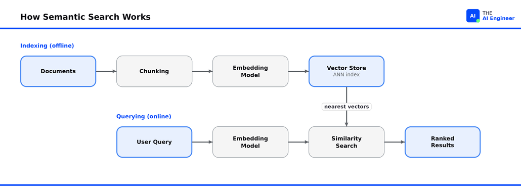
Indexing happens offline. Each document is chunked into retrievable units. Each chunk goes through an embedding model that turns text into a vector. Each vector is stored in a vector store with an approximate-nearest-neighbor index. Once indexed, documents are ready for any query. Each vector is stored in a vector store with an approximate-nearest-neighbor index.
🏗️ At Scale: The managed version of that vector store is its own product category. What Does Pinecone Actually Do? breaks down the best-known one.
Querying happens online. The query passes through the same embedding model and becomes a query vector. The system runs a similarity search (cosine, dot product, or Euclidean distance) to find the nearest document vectors. Results come back ranked by proximity.
The technique that made this practical is Sentence-BERT. The problem it solved was speed. The original BERT compared two sentences by running them through the model together, so finding the closest pair in 10,000 sentences meant about 65 hours of computation. Sentence-BERT encodes each sentence into a vector once, so search compares vectors: about 5 seconds for the same 10,000 pairs.
The 2026 Embedding Model Landscape
The embedding model is what turns meaning into geometry. It maps documents and queries into vectors, and how well it groups related meaning is the upper bound on retrieval quality. A weak model and the right document never makes it into the candidate set.
Models differ on four properties: retrieval accuracy on target domain (web prose, code, legal text, etc.), vector dimensionality (which sets storage and search cost), context length (how much text fits in one embedding), and how far they fall on domains they were not trained on. MTEB (the Massive Text Embedding Benchmark) scores embedding models across 56 English datasets in 8 task categories (retrieval, classification, clustering, reranking, and more), with a multilingual variant covering 250+ languages.
As of mid-2026 the leaderboard looks like this:
Google Gemini Embedding 001 leads English MTEB at mean task score 68.32,
OpenAI text-embedding-3-large is the closest commercial competitor at 64.6, with 3,072 dimensions, and the default if you are already on OpenAI infrastructure1.
Cohere Embed and Voyage are the strongest commercial options outside Google, and both sell domain-tuned variants (Cohere for multilingual, Voyage for code and finance).
Open-weight models have caught up: Qwen3-Embedding and BGE rank near the top of MTEB and can be self-hosted, so you pay no per-query fee and your data stays in-house.
One caveat the leaderboards do not make obvious: MTEB scores are self-reported. Providers submit their own numbers. There is no independent verification step. So a top MTEB rank tells you a model is worth testing, not that it will win on your data. Use the leaderboard to pick three or four candidates, then run them against your own documents and rank by MRR or NDCG@k before you commit.
Semantic Search in Production
Dense vectors generalize meaning, and that same strength is their weakness: they lose exact-match precision. Search for an error code like 0x80070005 or a specific SKU, and the vector lands in a fuzzy neighborhood of “things like this” instead of the exact string. BM25, the keyword-matching algorithm, nails those because it matches the literal token you typed. So the best production systems run both.
That combination is hybrid search: run BM25 and dense retrieval side by side, then merge the two ranked lists.
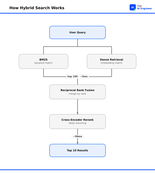
The standard way to merge them is Reciprocal Rank Fusion (RRF), which ranks a document by its position in each list instead of its raw score. Why position and not score? BM25 scores are unbounded while cosine similarities sit between -1 and 1, so averaging the two raw numbers is meaningless. Ranking by position sidesteps that, and rewards documents both methods rank highly.
The second universal addition is reranking, which exploits a difference between two model architectures. A bi-encoder (your embedding model) encodes the query and the document in two independent passes, which is fast and lets you precompute document embeddings. A cross-encoder runs the query and the document through the model together, so the model can weigh every word in the query against every word in the document at once. The cross-encoder is far more accurate, since it understands negation, comparison, and conditional logic, but it cannot be precomputed and runs one forward pass per pair.
The production pattern chains them. A bi-encoder retrieves the top 100 in ~5ms; a cross-encoder rescores those 100 in ~50ms; the reranked top 10 go to the application or LLM. For the reranker itself, Cohere Rerank is the standard hosted call and BGE Reranker is the standard self-hosted one.
Two limitations remain:
Out-of-domain failure is real. The BEIR benchmark exists to surface it: dense models trained on web text underperform zero-shot on biomedical, legal, financial, and tweet corpora. On BioASQ (biomedical literature) and Signal1M (tweets), BM25 actually beats most embedding APIs. Fine-tuning on domain data closes the gap, often by 10 to 30 percentage points for legal, medical, and code2.
Chunking is its own separate problem. Fixed-size chunking is the fast baseline but splits sentences mid-thought. Semantic chunking groups by meaning at higher compute cost. Hierarchical chunking embeds small precise child chunks but returns larger parent context to the LLM. No single strategy wins across corpora. You tune to your data.
Who Is Building This in Production
Spotify rebuilt podcast search around meaning. They trained an embedding model on (query, episode) pairs mined from real search logs, so a search like “podcasts about starting a business” matches a relevant show even when the title never uses those words. At query time, that model pulls the top semantic candidates from a vector index, and a final ranker blends their scores with Spotify’s existing keyword results. The architectural choice worth copying: they kept keyword search in the mix rather than replacing it. As ML engineer Alexandre Tamborrino put it, dense retrieval “often fails to perform as well as traditional IR methods on exact term matching.” Running both, the system lifted podcast engagement enough in an A/B test to roll out to most users3.
Notion runs semantic search under its AI Q&A feature, which answers natural-language questions across a user’s workspace and connected tools like Slack and Drive. Every page is chunked into spans, each span is embedded, and the vectors are stored with the page’s author and permission metadata attached. Over two years Notion scaled that vector search 10x while cutting cost roughly 90%, and the lesson is in how. Re-embedding every page on every edit would be ruinously expensive, so Notion hashes each span’s text and caches the hashes: an edit re-embeds only the spans whose text actually changed, and a permissions change skips embedding entirely to patch the metadata in place. That change-detection step alone cut indexed data volume 70%.4
Algolia sells hybrid search as a product, so a team can buy the BM25-plus-vector blend instead of building it. Their NeuralSearch runs both on every keystroke and merges the scores in real time. The case for it is the long tail: Algolia pegs vague, wordy queries (where keyword search whiffs) at over half of all searches. When Frasers Group switched its Missguided and Isawitfirst stores onto it, zero-result searches dropped about 65% and conversion rose up to 17%5.
Keyword Search and Semantic Search Work Together
Semantic search doesn’t replace keyword search. What it does is buy you a second relevance signal that catches the paraphrase, intent, and cross-language matches the card catalog can never see. The card catalog and the librarian work side by side: production systems fuse both signals with RRF and rerank the top results with a cross-encoder that reads each candidate against the query.
So when you build search, the question to ask isn’t “keyword or vectors?” It’s “what’s the cheapest way to run both and let a reranker sort it out?” Start with BM25 because it’s free and instant, add embeddings when exact-match stops being enough, and add a reranker when you can afford the 50ms. That order, in that sequence, is how you ship search that actually works.
💬 Curious: what’s the search stack you’re running in production today, and what was the failure mode that made you start looking at semantic? Reply or comment. The most common pattern becomes a Friday case study.
Where to Next?
📖 Go Deeper → Vector DB Showdown: Pinecone vs Weaviate vs Qdrant. Where your embeddings live at scale.
🔗 Go Simpler → What are Embeddings?. The prerequisite: how text becomes a vector.
🔀 Go Adjacent → How DoorDash Built Their RAG System. Hybrid retrieval in production at scale.
🗺️ If you are transitioning into AI engineering, How to Break Into AI Engineering in 2026 is the full roadmap on getting there.
🔜 Friday: How CodeRabbit Reviews Code at Scale. The multi-agent pipeline behind every PR review.
OpenAI, New Embedding Models and API Updates (Jan. 2024).
Notion Engineering, Two years of vector search at Notion (Feb. 2026).